A little over a month ago Rob Hyndman finished the 2nd edition of his open source book Forecasting: Principles and Practice. Take a look, it’s a fantastic introduction and companion to applied time series modeling using R.
It made me I rediscover the tslm()-function of the excellent forecast-library, which provides a convenient wrapper for linear models with timeseries-data. The function provides two shorthands to add trend- and season-variables as regressors, which is quite useful to avoid problems such as “spurious regression”. Let’s look at an example.
Query Google Trends
# devtools::install_github("PMassicotte/gtrendsR")
library(gtrendsR)
trends <- gtrends(c("frühling", "spring"), geo = c("DE"))
Google Trends can often serve as useful demo-data for timeseries-modelling and the gtrendsR-package by Philippe Massicotte and Dirk Eddelbuettel makes it easy to access this data-source. Here we ask for the (relative) weekly search volume for Germany for the past five years for the keywords “frühling” and “spring”. An englisch word and its german equivalent.
Explore and Decompose the Series
To explore the data we can transform the data into timeseries and look at their (classical) decomposition:
library(tidyverse)
library(forecast)
library(ggseas)  # install from https://github.com/ellisp/ggseas

# turn dataframe into timeseries
create_ts <- function(df, kw){
  df %>%
    pluck("interest_over_time") %>%
    filter(date    >= as.Date("2014-01-01"),
           keyword == kw) %>%
    with(ts(hits, start = c(2014, 1), frequency = 52))
}

fruehling  <- create_ts(trends, "frühling")
spring     <- create_ts(trends, "spring")

# compare decomposition for both time series
cbind(fruehling, spring) %>%
  ggseas::tsdf() %>%
  gather("series", "hits", -x) %>%
  ggseas::ggsdc(aes(x, hits, colour = series), method = "decompose") +
  geom_line() +
  labs(x = "time", y ="hits", title = "Decomposition of Search Traffic")
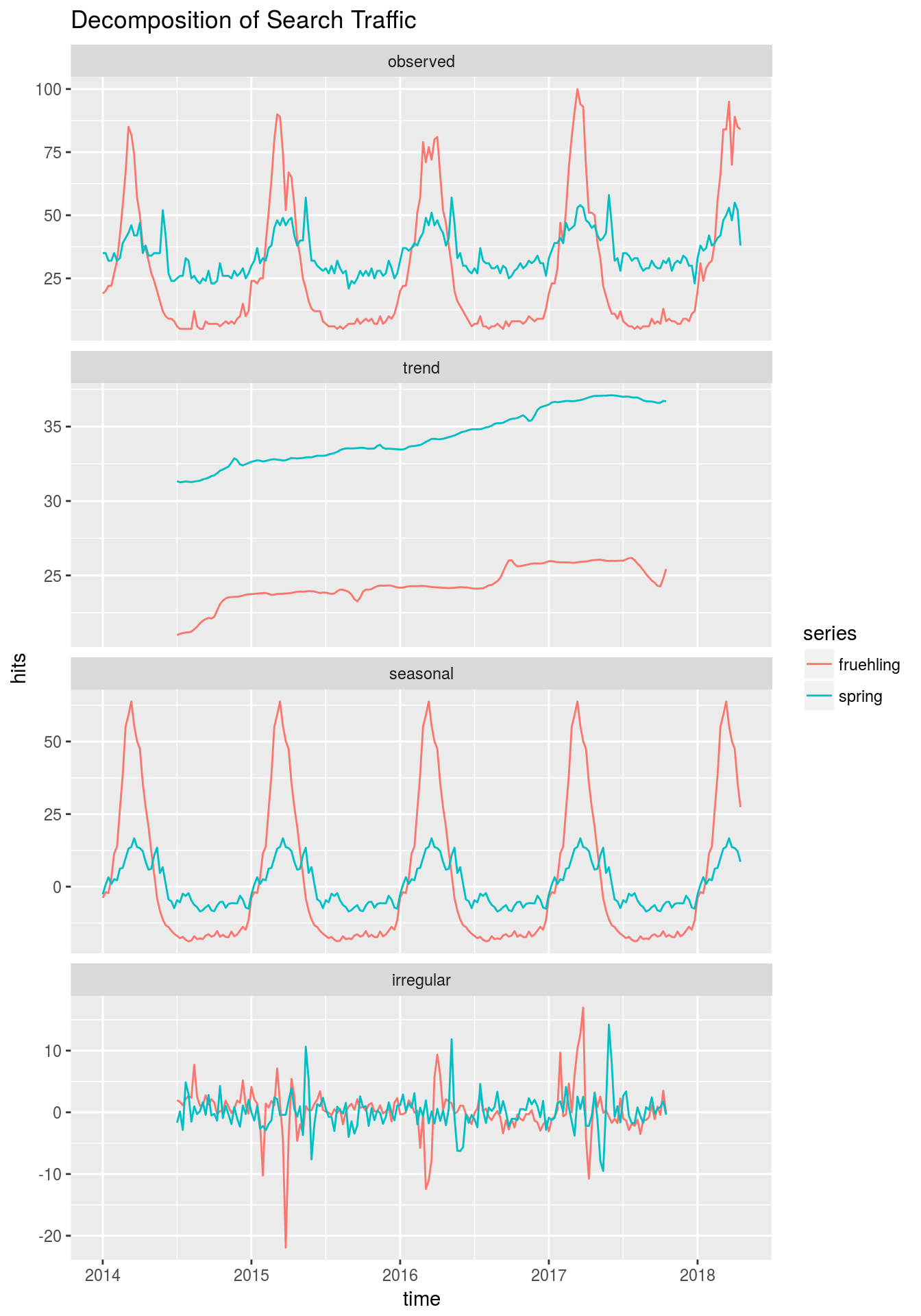
The overall search volume is higher for “frühling” than it is for “spring”. Both series show a seasonal pattern, while the search volume for “frühling” also shows a slight downwards trend - this may be influenced by a few bad springs which we had in Germany! :)
Model the Linear Relationship
Even though this is clearly seasonal data it may be useful to quantify the linear relationship between these two variables using linear regression. How strongly do the two search terms “swing together”?
But because the data is time-dependent and a least one series shows a trend, and both of them show a season, we should consider modeling these characteristics as well.
# customize model output
show_estimates <- function(model) {
  model %>%
    broom::tidy() %>%
    dplyr::select(term, estimate) %>%
    modify_if(is.numeric, round, 2) %>%
    # + some preparation to combine lm and arima output later
    modify_at("term", as.character) %>%
    modify_at("term", stringr::str_replace,
              pattern = "\\(Intercept\\)",
              replacement = "intercept") %>%
    modify_at("term", stringr::str_replace,
              pattern = "(trend|drift)", ## improve pattern
              replacement = "trend/drift")
}

#  customize html-tables
hux_table <- function(df, caption) {
  library(huxtable)

  content_rows <- 1:nrow(df) + 1  # +1 for the header
  content_cols <- 2:ncol(df)

  df %>%
    hux(add_colnames = TRUE) %>%
    set_bold(row = 1, col = everywhere, value = TRUE) %>%
    set_bottom_border(row = 1, col = everywhere, value = TRUE) %>%
    set_pad_decimal(content_rows, everywhere, ".") %>%
    set_align(c(1, content_rows), content_cols, "right") %>%
    set_number_format(content_rows, everywhere, "%5.4g") %>%
    set_caption(caption)
}
The above code is just to produce nicer outputs, show_estimates() serves as a customized version of broom::tidy() and hux_table() produces nice html-tables from a dataframe.
# fit models
ts_models <- list()
ts_models$lm1              <- tslm(fruehling ~ spring)
ts_models$lm1_trend        <- tslm(fruehling ~ trend + spring)

# inspect parameters
ts_models %>%
  map(show_estimates) %>%
  reduce(full_join, by = "term") %>%
  set_names(c("term", names(ts_models))) %>%
  filter(!str_detect(term, "season")) %>%
hux_table("Coefficients for Linear Models")| term | lm 1 | lm 1_trend |
| intercept | -61.35 | -59.26 |
| spring | 2.52 | 2.58 |
| trend/drift | -0.04 |
We can see, that the model with the trend produces similar estimates of the co-relation between the two series. In this case the model choice doesn’t seem to make that mucht of a difference, though the trend_model would probably be preferred. If the trend of the variables were stronger, the differences between the models would be bigger as well.
Accounting for Autocorrelation
Timeseries are often characterised by the presence of trend and/or seasonality, but there may be additional autocorrelation in the data, which can be accounted for. The forecast-package makes it easy to combine the time-dependent variation of (the residuals of) a timeseries and regression-modeling using the Arima or auto.arima-functions. (For the implementation details please see https://robjhyndman.com/hyndsight/arimax/.)
In this case, we will add an autocorrelation of order 1 to the model.
# fit regression with autocorrelated models
ts_models$ar1       <- Arima(fruehling, xreg = spring, order = c(1,0,0))
ts_models$ar1_trend <- Arima(fruehling, xreg = spring, order = c(1,0,0),
                             include.drift = TRUE)
# inspect parameters
ts_models %>%
  map(show_estimates) %>%
  reduce(full_join, by = "term") %>%
  set_names(c("term", names(ts_models))) %>%
  filter(!str_detect(term, "season")) %>%
hux_table("Coefficients including Autocorrelated Models")| term | lm 1 | lm 1_trend | ar 1 | ar 1_trend |
| intercept | -61.35 | -59.26 | 17.83 | 0.8 |
| spring | 2.52 | 2.58 | 0.39 | 0.39 |
| trend/drift | -0.04 | 0.15 | ||
| ar 1 | 0.97 | 0.96 |
Because our data shows a strong seasonal pattern, that hasn’t been accounted for in the regresssion model, the parameters of the AR-model differ strongly from the regression. This is because the AR-parameter picks up a lot of the seasonal variation in the data.
Summary
# compare models
ts_models %>%
  map_df(BIC) %>%
  gather("model", "fit") %>%
  arrange(fit) %>%
hux_table("Information Criteria")| model | fit |
| ar 1 | 1510 |
| ar 1_trend | 1514 |
| lm 1 | 1884 |
| lm 1_trend | 1884 |
The visual inspection of the data and the corresponding BIC-values indicate, that the ar1-model may be the model with the best fit and hence, the parameters of this model should be preferred to the other ones.
Overall I wanted to showcase some of tools one can use to analyze the relation between two timeseries and the implications of certain model choices. If you would like to read a little more about this topic, please take a look at the Regressions-Chapter of the fpp2-book. For comments and feedback on this post you can use the comments or reach me at twitter via @henningsway.